Questions for Week 6
During and after the lecture, I had a few questions that I think you’d find helpful too. So, I’ve put all the answers on here our website.
1) Why don’t we write z - w - k ?
The first question was: ’In the calculation of the surplus, why do we write z - w and not z - w - k?
Below is an intuitive explanation of why the free‐entry (zero‐profit) condition in the firm’s vacancy‐posting decision appears as
\underbrace{p_f}_{\text{Probability of success}}\;\times\;\underbrace{(z - w)}_{\text{Surplus per match}} \;-\; \underbrace{k}_{\text{Vacancy posting cost}} \;=\;0 \quad\Longleftrightarrow\quad p_f\,(z - w)\;=\;k,
and why we do not write the firm’s per‐match surplus as (z - w - k).
Short Answer: surplus vs. upfront cost
In a search and matching model (Diamond–Mortensen–Pissarides style), a firm:
- Pays an upfront cost k to create and maintain a vacancy (e.g., job ads, screening, overheads).
- Earns a flow surplus of \bigl(z - w\bigr) once a match is formed (productivity z minus the wage w).
Key point: The cost k is not part of the ongoing surplus from producing with the worker—it is an entry or vacancy‐posting cost. Once the firm has successfully matched with a worker, the firm gets instantaneous payoff z-w from that job. That’s why the firm’s surplus from an existing match is \boxed{z - w}, not \,(z - w - k).
If this is still not clear, lets look at the following details:
a) Expected payoff from posting a vacancy
Even though k is not subtracted each instant from the firm’s flow surplus, the firm must still consider k when deciding whether to post a vacancy. The probability of successfully filling a vacancy is p_f. Hence the expected net gain from posting one vacancy is:
\text{(Probability of success)}\;\times\;\text{(Surplus if successful)} \;-\; \text{(Cost of posting)}.
In symbols:
\underbrace{p_f}_{\text{Probability}} \times \underbrace{(z - w)}_{\text{Surplus per match}} \;-\; \underbrace{k}_{\text{Posting cost}}.
b) Zero‐profit (free‐entry) condition
In equilibrium with free entry of firms:
If the expected payoff were positive, more firms would enter (post vacancies). If it were negative, firms would exit.
Thus, in equilibrium, the expected net payoff must be zero.
Therefore we set
p_f\,\bigl(z - w\bigr) - k \;=\; 0 \quad\Longrightarrow\quad p_f\,(z - w) \;=\; k.
This is not saying the firm literally takes (z - w - k) each period as a flow payoff; it’s saying \boxed{\text{Expected Gain} - \text{Cost} = 0}.
c) Why we don’t write z - w - k
- Different time dimensions:
- z-w is a flow surplus once matched.
- k is typically an upfront or per‐period cost to keep the vacancy open.
- z-w is a flow surplus once matched.
- Surplus from a matched job:
- Once the firm has matched with a worker, the payoff in that match each instant is z - w. There’s no (-k) inside that flow because k is not being spent repeatedly; it was spent to create the vacancy.
- Expected value logic:
- The ex ante condition says “\mathrm{Probability} \times \mathrm{(Match~Surplus)} - \mathrm{Cost} = 0.”
- If we incorrectly wrote “(z - w - k)” as the firm’s match surplus, we’d be double‐counting k. The cost k is paid once per vacancy, not subtracted from the flow of production after the match is formed.
- The ex ante condition says “\mathrm{Probability} \times \mathrm{(Match~Surplus)} - \mathrm{Cost} = 0.”
Hence, z-w is the appropriate firm surplus per match, while k enters only in the entry or posting decision condition.
2) Is there a systematic strategy for solving comparative statics in the DMP Model?
As in many answer in economics the answer is: “it depends”.
But in this case, we might say yes. Below is a general strategy for performing comparative‐static exercises in a search‐and‐matching (DMP) framework. It’s typically more straightforward to start with the firm side (the free‐entry condition) and see how it affects labour‐market tightness j. Then we see how the resulting change in j feeds back into worker behavior, wages, and finally the full equilibrium.
a) The three building blocks in DMP
- Free‐Entry (Firm) Condition
- A firm posts a vacancy at cost k.
- The probability of filling that vacancy is p_f(j).
- Once matched, the firm’s per‐period payoff is (z - w).
- Zero‐profit (free entry) condition:
p_f(j)\,\bigl[z - w\bigr] \;=\; k, or in lecture slides we used the version below (same thing), e\,m\Bigl(\tfrac{1}{j},1\Bigr)\,\bigl[(1-a)(z-b)\bigr] \;=\; k. (The expression (1-a)(z-b) is the firm’s share of the total match surplus under Nash bargaining.)
- A firm posts a vacancy at cost k.
- Wage (Worker) Condition
- By Nash bargaining (or some other rule), the wage w depends on productivity z, unemployment benefit b, and the worker’s bargaining power a.
- Often it takes the form:
w \;=\; b \;+\; a\,(z - b). - This ensures the worker gets fraction a of the surplus (z - b).
- By Nash bargaining (or some other rule), the wage w depends on productivity z, unemployment benefit b, and the worker’s bargaining power a.
- Matching Function / Job Finding
- The probability a worker finds a job is p_c(j) (as a function of labour market tightness j), and the probability a firm fills a vacancy is p_f(j).
- The ratio of vacancies to unemployed is j. Typically, p_c(j) is increasing in j, while p_f(j) is decreasing in j.
- The probability a worker finds a job is p_c(j) (as a function of labour market tightness j), and the probability a firm fills a vacancy is p_f(j).
Putting these together, we solve for the equilibrium \{j, w, u, Y\}.
b) Why start with the firm side?
When we do a comparative‐static (like “What if k decreases?” or “What if z increases?”), the free‐entry condition often gives the most direct handle on how labour‐market tightness j adjusts. Once j is pinned down, you see how that affects:
- The job‐finding rate p_c(j), which influences unemployment.
- The vacancy‐filling rate p_f(j).
- Then, combined with the wage equation, you get the new equilibrium wage or payoff for workers.
Example: If k Decreases
- Firm Behavior:
- The zero‐profit condition is p_f(j)\,(z - w) = k.
- A decrease in k means that if j stayed the same, the left side p_f(j)\,(z - w) would be bigger than the cost. Firms would make a positive profit.
- Hence new firms enter (post more vacancies), so j (vacancies/unemployed) goes up.
- The zero‐profit condition is p_f(j)\,(z - w) = k.
- Worker Side:
- As j rises, the job‐finding rate p_c(j) also rises.
- This might affect worker surpluses (since it’s now easier to find a job, workers’ fallback unemployment is less “painful”). That in turn might feed back into wage bargaining, depending on the exact wage equation.
- As j rises, the job‐finding rate p_c(j) also rises.
- Overall Equilibrium:
- We find the new j that satisfies the free‐entry condition with the new cost k.
- We combine that with the wage equation w = b + a(z - b) (or any wage equation that might itself depend on j, if the model does so).
- Finally, from the new j, we infer unemployment u via u = 1 - p_c(j).
- We find the new j that satisfies the free‐entry condition with the new cost k.
So the chain is often:
(1) Free‐entry → (2) Solve for j → (3) See effect on wages & unemployment.
c) Why not start with the worker side?
We could start by writing down the worker’s job‐finding probability, or the wage equation, and see how it changes with z or k. However:
- The worker side typically doesn’t determine j by itself.
- The worker’s payoff from searching or the wage often depends on firms’ vacancy decisions (which is captured by j).
- It’s more natural to see how changes in k, z, or b shift the firm’s incentives to post vacancies, which directly changes j.
- Then we feed that back into the worker side (bargaining or job‐finding rates).
In short, the firm’s free‐entry condition is usually the “bottleneck” that pins down how many vacancies get created. That sets the labour‐market tightness. Then, from that tightness, we see how quickly workers find jobs and what the equilibrium wage is.
d) General comparative‐static steps
Here’s a systematic approach to any parameter change:
- Identify which equation(s) the parameter appears in:
- For instance, if z (productivity) changes, it appears in both the firm’s surplus (z - w) and the wage equation w = b + a(z-b).
- If k changes, it directly appears in the free‐entry condition.
- For instance, if z (productivity) changes, it appears in both the firm’s surplus (z - w) and the wage equation w = b + a(z-b).
- See how the free‐entry condition is altered:
- Typically, something on the left side \bigl[p_f(j)\,(z - w)\bigr] must adjust to keep it equal to k.
- This drives a change in j.
- Typically, something on the left side \bigl[p_f(j)\,(z - w)\bigr] must adjust to keep it equal to k.
- Deduce how j changes:
- If k goes down, we expect more vacancies → j goes up.
- If z goes up, the firm’s surplus (z - w) is bigger, so we expect more entry → j goes up (unless wage also rises enough to offset it).
- If k goes down, we expect more vacancies → j goes up.
- Check the wage or worker payoff side:
- If wage depends on z, it might rise. If wage is partly a function of j (some models have that), it might also respond.
- Determine final outcomes \{j^*, w^*, u^*, Y^*\}.
e) Concluding remarks
- Yes, the standard approach is:
- Look at firm behavior (free entry) → figure out how j changes.
- Then see how that new j affects worker outcomes, wages, and unemployment.
- Look at firm behavior (free entry) → figure out how j changes.
- We do it this way because firm entry is typically the driving force behind labour‐market tightness, which in turn determines job‐finding rates and shapes worker payoffs.
3) Why is the Walrasian wage above the worker’s effort cost?
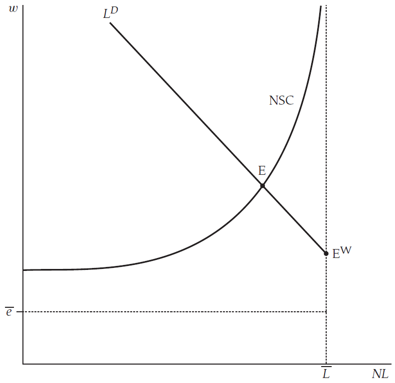
In lecture slides page 52 (or David Romer Advanced Macroeconomics 5^th Edition page 537) there is a diagram that shows the Walrasian equilibrium wage (E^W) is above the worker’s effort cost (\bar{e}).
What would happen if the detection rate q \to \infty? Should the Walrasian wage be equal to the worker’s effort cost? Why not? Why is it above in the diagram?
a) Distinguishing Between \bar{e} and the Walrasian Wage
Let’s first define the two concepts again:
\bar{e} = the worker’s cost of effort (disutility).
This is how much disutility or “effort cost” a worker experiences when working (spending time and resources etc on the job). It is not necessarily the “opportunity cost” or “reservation wage” from the worker’s perspective in a standard supply‐demand sense; it’s simply the cost in utility terms for supplying effort.E^W = the Walrasian (competitive) wage
This is the wage that would arise if there were no frictions, no moral hazard (so no efficiency wage), and if labour supply were fully employed. Mathematically, it typically comes from “\text{marginal~product~of~labour} = \text{wage}” at full employment (or at the intersection of labour supply and labour demand).
Hence, there is no reason in a standard neoclassical setting that E^W must equal \bar{e}. In fact, if the marginal product of labour at full employment is larger than \bar{e}, then the Walrasian wage is above \bar{e}.
Example: “Marginal Product” vs. “Effort Cost”
- Suppose the production function is such that at full employment (L = \bar{L}), the marginal product of an additional worker is still above \bar{e}. Then in a frictionless, competitive market, the wage is pinned down by that marginal product—not by the worker’s disutility.
- Graphically, if the labour supply is inelastic (vertical at \bar{L}), the wage is the height of the labour demand curve at \bar{L}. If that height is bigger than \bar{e}, the Walrasian wage E^W is above \bar{e}.
b) Why “as q \to \infty, w \to \bar{e}” in the no‐shirking condition
In the Shapiro–Stiglitz model with a “no‐shirking condition” (NSC), the wage needed to deter shirking is:
w_{\text{NSC}} \;=\; \bar{e} \;+\; \left(\rho \;+\; \frac{\bar{L}}{\bar{L} - N L}\,b\right)\,\frac{\bar{e}}{q}.
When the detection rate q \to \infty, the “incentive premium” \left(\rho + \frac{\bar{L}}{\bar{L}-N L} b\right)\frac{\bar{e}}{q} goes to zero, so the no‐shirking wage w_{\text{NSC}} goes to \bar{e}.
Interpretation: If firms can detect shirking instantly (q extremely large), workers can’t get away with slacking off. Hence, the extra wage premium to induce effort collapses, so the “efficiency wage” portion disappears.
Careful: This does Not force the Walrasian wage to equal \bar{e}
When q\to\infty, the no‐shirking constraint becomes irrelevant—but that does not mean the entire labour market sets w = \bar{e}. The Shapiro–Stiglitz model says:
- Without moral hazard, the market would go to the standard competitive outcome:
- Firms set “\text{marginal product} = \text{wage}.”
- All workers are employed if the marginal product is still above \bar{e} at \bar{L}.
- Firms set “\text{marginal product} = \text{wage}.”
Thus, if at full employment the marginal product is greater than \bar{e}, the Walrasian wage is above \bar{e}. This is exactly what David Romer’s figure shows: the point E^W is typically somewhere above the line \bar{e}. (otherwise why would workers work if they are paid \bar{e}?)
In other words, the condition “w_{\text{NSC}} \to \bar{e}” as q \to \infty just means the “efficiency wage premium” goes to zero. But the actual equilibrium wage in a frictionless (Walrasian) world is determined by supply–demand fundamentals, not by \bar{e}.
c) Putting it all together (mathematically and graphically)
- Walrasian model (no monitoring problem):
- Equilibrium wage = marginal product at full employment.
- If that marginal product is, say, > \bar{e}, then E^W > \bar{e}.
- Equilibrium wage = marginal product at full employment.
- Shapiro–Stiglitz (with monitoring problem):
- If q is finite, the no‐shirking condition requires a wage above \bar{e} by some premium.
- Equilibrium unemployment arises because that wage is higher than the Walrasian level, or at least above the competitive clearing wage.
- If q is finite, the no‐shirking condition requires a wage above \bar{e} by some premium.
- As q \to \infty:
- The no‐shirking constraint “collapses” to w_{\text{NSC}} = \bar{e}.
- But the actual frictionless equilibrium wage (the Walrasian wage) may well be some other value (likely above \bar{e} if the marginal product is bigger).
- The difference is that now moral hazard is no longer a constraint, so the wage is set purely by standard supply–demand. That standard supply–demand outcome is typically above \bar{e} if the marginal product at full employment is above \bar{e}.
- The no‐shirking constraint “collapses” to w_{\text{NSC}} = \bar{e}.
Hence, in Romer’s diagram, the point labeled E^W (the Walrasian or “no‐monitoring‐problem” equilibrium) is usually drawn above \bar{e}. The model’s statement that w \to \bar{e} as q \to \infty refers specifically to the NSC line going downward and losing its force, not to the entire labour market wage necessarily equaling \bar{e}.
Summary
- Cost of effort vs. Competitive wage: Just because it costs a worker \bar{e} in effort does not mean the “market wage” is \bar{e}. The market wage is typically set by productivity (and possibly by supply–demand conditions), which can easily exceed \bar{e}.
- q \to \infty Kills the efficiency‐wage premium: A very high detection rate means the “extra” wage needed to prevent shirking is effectively zero, so the “efficiency wage” effect vanishes. That drives the NSC wage formula down to \bar{e}.
- But the frictionless, Walrasian wage is not pinned to \bar{e}; it is pinned to the marginal product at full employment, which can be bigger (thus E^W is above \bar{e} in the figure).
Thus, in Romer’s figure the point labeled “E^W” is the wage–employment outcome if the moral hazard problem disappeared. Since the production function might be quite productive, that wage can be strictly above the cost of effort \bar{e}.